Argmax on a 2D polytope

Select the best vertex of a random convex polytope in 2D: predict a cost direction θ from features, then return the vertex v maximizing θᵀv. The 2D setting makes this benchmark visual: the cost direction and selected vertex can be plotted directly, and the loss landscape can be shown as a contour plot over the 2D θ space.

using DecisionFocusedLearningBenchmarks
using Plots

b = Argmax2DBenchmark(; seed=0)

Argmax2DBenchmark(nb_features=5)

Observable input

At inference time the decision-maker observes the feature vector x and the polytope shape, but not the cost direction hidden θ:

dataset = generate_dataset(b, 50; seed=0)
sample = first(dataset)
plot_context(b, sample)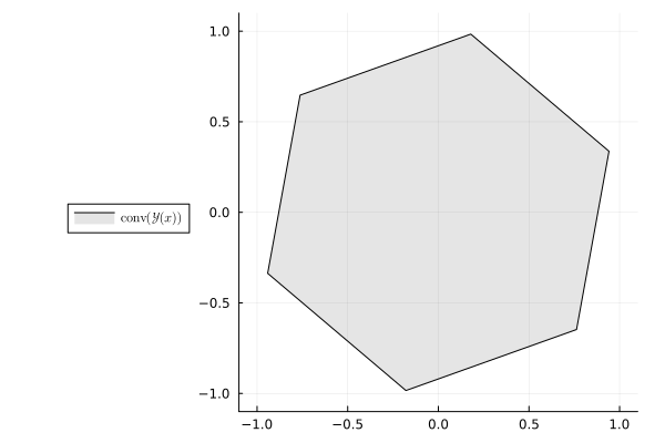

A training sample

Each sample is a labeled triple (x, θ, y):

• x: feature vector (observable at train and test time)
• θ: 2D cost direction (training supervision only, hidden at test time)
• y: polytope vertex maximizing θᵀv (optimal decision)
• instance (in context): polytope vertices (observable problem structure)

The full training triple (polytope, cost direction θ, optimal vertex y):

plot_sample(b, sample)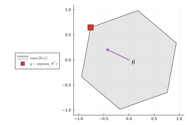

Untrained policy

A DFL policy chains two components: a statistical model predicting a 2D cost direction:

model = generate_statistical_model(b)     # linear map: features → 2D cost vector

Dense(5 => 2; bias=false)  # 10 parameters

and a maximizer selecting the best polytope vertex for that direction:

maximizer = generate_maximizer(b)         # vertex maximizing θᵀv over polytope vertices

maximizer (generic function with 1 method)

A randomly initialized policy predicts an arbitrary cost direction:

θ_pred = model(sample.x)
y_pred = maximizer(θ_pred; sample.context...)
plot_sample(b, DataSample(sample; θ=θ_pred, y=y_pred))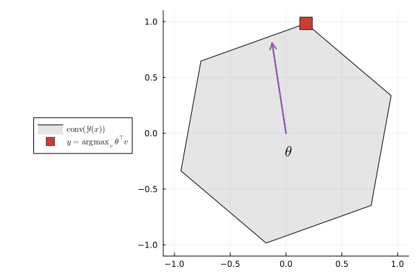

Problem Description

In the Argmax2D benchmark, each instance defines a random convex polytope $\mathcal{Y}(x) = \mathrm{conv}(v_1, \ldots, v_m)$ in $\mathbb{R}^2$. A hidden encoder maps features $x \in \mathbb{R}^p$ to a 2D cost vector $\theta \in \mathbb{R}^2$. The task is to find the polytope vertex maximizing the dot product:

\[y^* = \mathop{\mathrm{argmax}}\limits_{v \in \mathcal{Y}(x)} \; \theta^\top v\]

This is a toy 2D combinatorial optimization problem useful for visualizing how well a model learns the cost direction.

Key Parameters

DFL Policy

\[\xrightarrow[\text{Features}]{x} \fbox{Linear model} \xrightarrow{\theta \in \mathbb{R}^2} \fbox{Polytope argmax} \xrightarrow{y}\]

Model: Dense(nb_features → 2; bias=false): predicts a 2D cost direction.

Maximizer: finds the vertex of the instance polytope with maximum dot product with θ.

This page was generated using Literate.jl.