Stochastic Vehicle Scheduling

Assign vehicles to cover a set of tasks while minimizing costs under stochastic delays: the DFL agent learns to predict adjusted costs that implicitly hedge against uncertainty.

using DecisionFocusedLearningBenchmarks
using Plots

b = StochasticVehicleSchedulingBenchmark(; nb_tasks=10)

StochasticVehicleSchedulingBenchmark(10, 10)

Observable input

Each instance is a city with task locations and scheduled times. Task spatial positions and scheduled times are observable at inference time. store_city=true is required to visualize the map (not needed for training):

sample = generate_dataset(b, 1; store_city=true)[1]
plot_context(b, sample)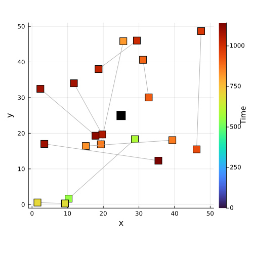

A training sample

Each sample is a labeled triple (x, θ, y):

• x: 20-dimensional feature vector per edge, encoding schedule slack and travel times
• θ: adjusted edge costs (training supervision only, hidden at test time)
• y: binary assignment (y[(u,v)] = 1 if a vehicle travels edge (u, v) in the schedule)

Unlike static benchmarks, y labels are not available by default and must be attached via a target_policy (e.g., the deterministic VSP solver). Routes are visualized in the untrained policy section below.

Untrained policy

A DFL policy chains two components: a statistical model predicting adjusted edge costs:

model = generate_statistical_model(b)     # linear map: task features -> adjusted edge costs

Chain(
  Dense(20 => 1; bias=false),           # 20 parameters
  vec,
) 

and a maximizer solving the deterministic VSP given those costs:

maximizer = generate_maximizer(b)         # deterministic VSP solver (HiGHS MIP)

DecisionFocusedLearningBenchmarks.StochasticVehicleScheduling.StochasticVechicleSchedulingMaximizer{typeof(DecisionFocusedLearningBenchmarks.Utils.highs_model)}(DecisionFocusedLearningBenchmarks.Utils.highs_model)

The untrained model predicts random edge costs; the resulting schedule is arbitrary:

θ_pred = model(sample.x)
y_pred = maximizer(θ_pred; sample.context...)
plot_sample(b, DataSample(sample; θ=θ_pred, y=y_pred))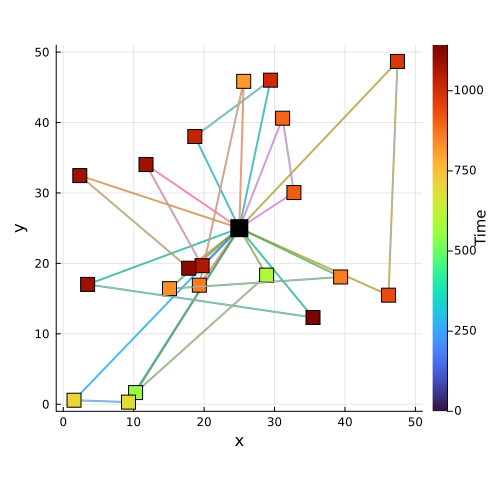

Problem Description

Overview

In the Vehicle Scheduling Problem (VSP), we consider a set of tasks $V$. Each task $v \in V$ has a scheduled beginning time $t_v^b$ and end time $t_v^e$, with $t_v^e > t_v^b$. We denote $t^{tr}_{(u,v)}$ the travel time from task $u$ to task $v$. A task $v$ can follow $u$ only if:

\[t_v^b \geq t_u^e + t^{tr}_{(u,v)}\]

An instance of VSP can be modeled as an acyclic directed graph where nodes are tasks and edges represent feasible successions. A solution is a set of disjoint paths such that all tasks are fulfilled exactly once to minimize total costs.

In the Stochastic VSP (StoVSP), after the scheduling decision is set, random delays propagate along vehicle tours. The objective becomes minimizing base costs plus expected total delay costs over scenarios.

Mathematical Formulation

Variables: Let $y_{u,v} \in \{0,1\}$ indicate if a vehicle performs task $v$ immediately after task $u$.

Delay Propagation: For each task $v$ in scenario $s$:

• $\gamma_v^s$: intrinsic delay of task $v$
• $d_v^s$: total accumulated delay
• $\delta_{u,v}^s = t_v^b - (t_u^e + t^{tr}_{(u,v)})$: slack time

\[d_v^s = \gamma_v^s + \max(d_u^s - \delta_{u,v}^s,\; 0)\]

Objective:

\[\min_{y} \; \sum_{(u,v)} c_{u,v} \, y_{u,v} + \mathbb{E}_{s \in S}\!\left[\sum_v C_d \, d_v^s\right]\]

Key Components

StochasticVehicleSchedulingBenchmark

Instance Generation

Each instance simulates a geographic city with depots and task locations. Tasks have realistic scheduled start/end times. Scenarios are random intrinsic delays $\gamma$ drawn from a Log-Normal distribution. Feature vectors are 20-dimensional.

Baseline Policies

DFL Policy

\[\xrightarrow[\text{Features}]{x \in \mathbb{R}^{20}} \fbox{Linear model $\varphi_w$} \xrightarrow[\text{Predicted cost}]{c} \fbox{Deterministic VSP solver} \xrightarrow[\text{Routes}]{y}\]

By training end-to-end with the deterministic solver, the linear model learns adjusted costs $c$ that implicitly account for expected stochastic delays, while keeping the fast deterministic solver at inference time.

Model: Chain(Dense(20 -> 1; bias=false), vec): predicts one adjusted cost per edge.

Maximizer: StochasticVehicleSchedulingMaximizer: HiGHS MIP solver on the deterministic VSP instance.

This page was generated using Literate.jl.